Our team have been using connected vehicle data from multiple suppliers since 2018 and it has transformed how we understand traffic and safety. It can show how fast vehicles are moving on almost every road, without the need for costly roadside sensors or repeated surveys, often with the ability to unlock data from over a decade ago. That level of coverage is a major step forward for anyone working in road safety, transport planning or network management.
However, there is an important constraint sitting behind all this capability. Connected vehicle data can only ever provide a sample, not a 100% census, which has consequences for what it can and cannot reliably measure. Together with our team of statisticians and data scientists we have been investigating this.
Let's consider two common scenarios. In the first, an authority wants to understand typical speeds on a residential road. The road carries relatively low traffic, perhaps only a few hundred vehicles per hour at peak. Looking at any single-hour window with a low-sample-size dataset will yield little or no usable information. There aren't enough observed vehicles to produce a reliable estimate.
In the second scenario, a scheme has been introduced on a busy urban corridor, and the question is how speeds have changed from one week to the next. Here, traffic volumes are high, but the timeframe is short. Again, the sample size becomes the main problem. Even on a busy road, a small percentage of vehicles observed over a single week may not be enough to reliably detect change, especially if the changes themselves are modest.
In both cases, the data exists. The question is whether it is large enough to support the conclusion being asked of it.
Connected vehicle data does not observe every vehicle on the road. It captures those that happen to be connected at that moment, creating a slice of the traffic stream rather than a complete picture. Depending on the provider and location, that slice typically represents about 1% to 25% of vehicles, often at the lower end of that range. Published studies put usable floating car penetration in the 1% to 5% range for many networks, rising to 10% to 15% in some dense urban areas, although we do work with suppliers who exceed this in their more recent data. This variation matters because the size of that slice directly determines how reliable any resulting insight will be.
Consider a single-hour window on a moderately busy road carrying 800 vehicles per hour. At a 1% sample, around 8 vehicles are observed. On a quieter residential street, there may be no observations at all.
A useful way to think about this is through the analogy of an exit poll. Pollsters don't ask every voter how they voted; they ask a sample and infer the overall result. A well-designed poll based on a few thousand responses can predict a national outcome with a high degree of accuracy. But asking five people in a single village tells you very little. Connected vehicle data works in the same way. The reliability of the result depends not on the existence of data, but on how many observations underlie it at a given place and time.
At Agilysis, we have worked extensively with multiple connected vehicle data suppliers over the last eight years. These datasets draw on a combination of embedded vehicle systems, aftermarket telematics and tracking devices, and mobile applications. Each source contributes differently to the overall sample, which means penetration rates vary, and so does the level of confidence that can be applied to the results. What determines whether an analysis is robust is not just where the data comes from, but how much of it there is.
Low Sample Sizes: What is the reliability problem?
When sample sizes are small, the only way to build confidence is through accumulation. A 1% sample observed over a single day is extremely limited. The same 1% sample observed over a full year adds reliability. Returning to the earlier residential road example, pooling data across 365 days transforms a handful of observations per day into a dataset that supports statistically robust analysis.
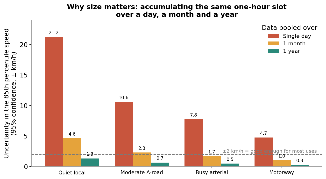
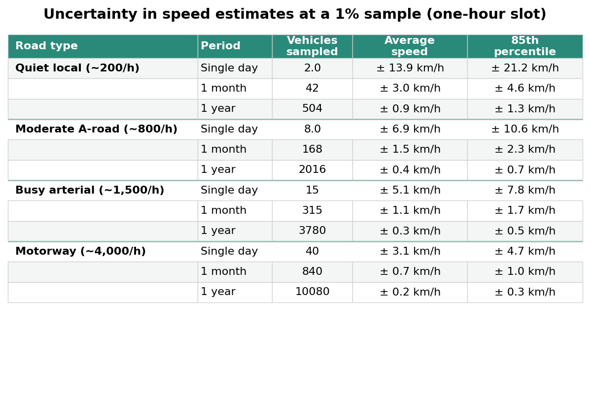
However, this does not remove the underlying limitations. As the time window narrows, the sample size decreases again. When the same data is broken down into shorter periods, such as a single hour shown in the table and chart on this page, the number of observations falls. On higher-flow roads, there may still be enough data to produce a stable average speed. On lower-flow roads, the numbers fall away quickly. In these situations, presenting a precise figure risks creating a false sense of accuracy. A number may look authoritative regardless of how many observations it is based on, but if the sample is too small, the result is inherently unreliable.
This becomes more apparent when comparing averages and percentiles. Suppose you want to estimate the average speed and 85th percentile speed for a single road segment. Consider a single-hour window on a moderately busy road carrying 800 vehicles per hour. At a 1% sample, around 8 vehicles are observed. On a quieter residential street, there may be no observations at all. Eight vehicles are not enough to confidently describe the behaviour of 800.
The issue becomes more significant when calculating the 85th percentile, which depends on identifying the faster end of the speed distribution. If, for example, estimating the average required about 100 vehicles, then estimating the 85th percentile would need about 225 vehicles, more than double. Still, this would only get you to a rough figure with a reliability of ±2kph (1.3mph). The 85th percentile is inherently more sensitive because it focuses on the extremes rather than the centre. With too few observations, small variations in the sample can lead to large changes in the result. Having a number is not the same as having a trustworthy number.
If the requirement is to understand what is happening over a short period, such as assessing the impact of a change from one week to the next, waiting to build a larger sample over months or years is not practical. In these cases, the only way to increase confidence is to use a larger dataset.
How Larger Samples Transform Data Reliability
The data we use from TomTom is estimated to capture between 23% and 33% of vehicles on the road. At this level, the number of recorded vehicles increases significantly. The same road, carrying 800 vehicles per hour, no longer yields a single-digit sample; it gives around 240 observed vehicles over the same period. Over just a few hours, this builds into a large, stable dataset that can support much more precise analysis and evaluation. Questions that can't be answered with a 1% sample become entirely feasible.
Small sample datasets, when accumulated over long periods, are well-suited to understanding typical conditions across a network. We use some small sample size data to look at all-day average speeds on relatively low-flow roads with no problem, but we are also only doing this for a whole year. We take care to assess all of the data we use and protect clients from seeing unreliable data.
Higher-sample datasets, even over shorter periods, support more detailed, time-sensitive analysis. The critical factor is ensuring that the sample size matches what you're trying to achieve. Without understanding the underlying sample size, it is easy to over-interpret what the data is actually showing.
For analysts and road safety practitioners, this distinction is critical. It influences whether conclusions are robust or fragile, whether interventions are well-targeted or misdirected, and whether decisions are based on evidence or assumption. Connected vehicle data provides unprecedented coverage and has fundamentally improved what can be measured across a network, but it does not remove the need for careful interpretation.
The question is no longer simply whether data is available. It is whether there is enough of it to make it meaningful.

CEO
Richard Owen

Principal Consultant
Nathan Harpham

Marketing Manger